This note details methods to solve continuous time optimization problems using the Hamiltonian and the Maximum Principle. These are just a typeset version of the notes I made while studying, using the material from lecture notes and figuring out the details (primarily typo resolution). Apologies if I made any errors of my own.
where x∈Rm is a state vector and u∈Rn is a control vector. For any function f:X×Y→Rk, fx(x,y) denotes the partial derivative of f with respect to x. If x is a vector in Rn, then fx(x,y) is a n×k matrix. For any function of time, f˙(t) is its time derivative. If f is a column vector, so is f˙(t).
Consider the Lagrangian approach to solving problem (1). For each period t, we have a constraint g(x(t),u(t))−x˙(t)=0. We can rewrite this as e−ρt(g(x(t),u(t))−x˙(t))=0. Then, the Lagrangian for this problem is defined as
The time-varying Lagrange multipliers, λ(t), are referred to as the co-state variable. Pontryagin’s maximum principle provides an alternative approach to solving this optimization problem. To do so, we must first define the Hamiltonian function, H:Rm×Rn×Rm→R, defined as:
The maximum principle characterizes a collection of first-order necessary conditions that must be satisfied by the optimal solution to problem (1).
Caution: differentiating the maximized Hamiltonian
Using the first order conditions, we defined u∗(x,λ) and the maximized Hamiltonian H∗(x,λ)=H(x,u∗(x,λ),λ). We start from Hu(x,u∗(x,λ),λ)=hu(x,u∗(x,λ))+gu(x,u∗(x,λ))λ=0. Hu is an n×1 vector, so Hux and Huλ are n×m matrices. The (dimension-corrected) formulae for these matrices, as in the lecture notes, are
Unfortunately, gu was already an m×n matrix, so the term guu or gux is not well-defined as a matrix in the usual sense. The derivative of guλ, which is an n×1 vector, is still well-defined as an m×n matrix, so the operation itself is not inappropriate. These problems will not arise when the state or control are scalars, and I’m sure there is some correct way of defining these higher-order derivatives.
With the expressions for the derivatives defined as they are here, we can reconcile the steady-state formulae for the system. From the dynamical system governing the evolution of the costate and state variables, the steady state is defined as
The steady state can then be shown to be characterized by
f′(k)cλ=ρ+δ=f(k)−δk=U′(c)
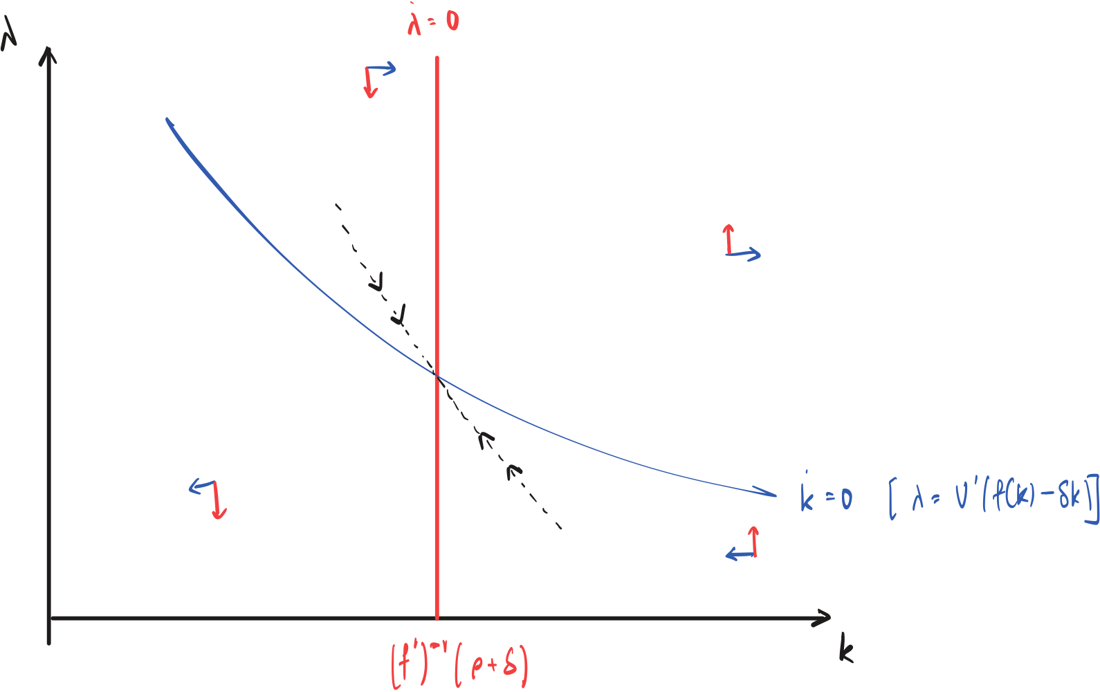
The dynamical system of (λ,k) can be written, using the optimal decision rule, as
λ˙=λ[ρ+δ−f′(k)]k˙=f(k)−δk−(U′)−1(λ)
with the corresponding phase diagram below.
Neoclassical growth
Then, to linearize the system around the steady state, we use a Taylor expansion and the Envelope theorem (to use derivatives from the maximized Hamiltonian). The non-linear system is
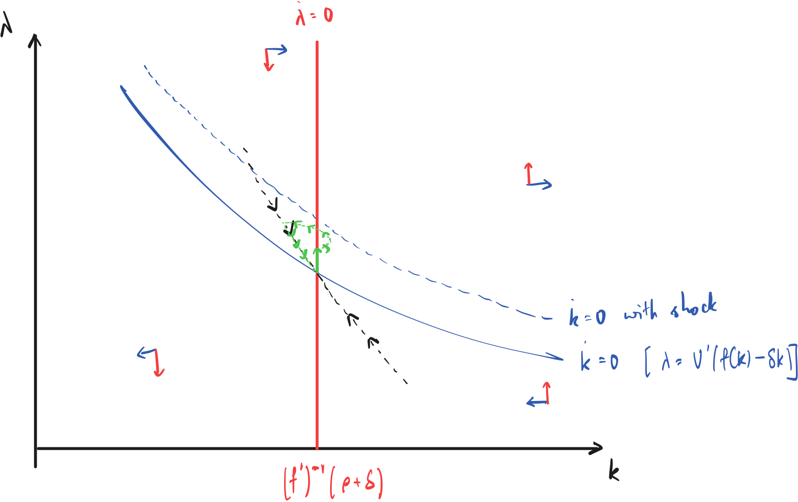
Consider a news shock about temporarily low productivity in the future in the neoclassical growth model above. The response, due to the smoothing motive, would be a fall in consumption today, which leads to a corresponding increase in the co-state. We can use the phase diagram then to analyze the path of the economy back to the steady state.
Response to a news shock
After the initial upward jump in the costate, the costate and capital stock increase, following the evolution equations for the neoclassical growth model. However, at the point when the shock arrives, the production function changes from f to f~ which has a lower marginal product of capital uniformly. When the productivity change takes effect, capital stock begins to decline as the k˙ is determined by the new production function, with the k˙=0 locus being the dotted line in the phase diagram. As the shock dissipates, the economy returns to the saddle path, and returns to the steady state thereafter.
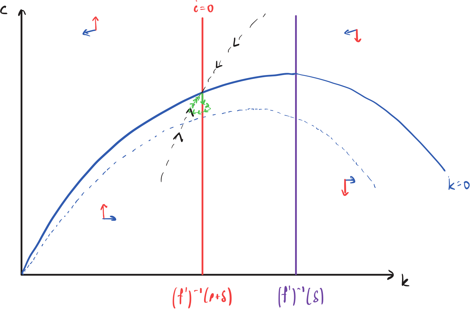
In this model, we can alternatively analyze the impact of the shock by looking at a system of (c,k) instead of (λ,k) due to a one-to-one correspondence between c and λ. Using U′(c)=λ, write λ˙=U′′(c)c˙. Then,
c˙(t)=−U′′(c)U′(c)[f′(k)−δ−ρ]
Then, consumption falls when f′(k)<ρ+δ and increases otherwise. The same news shock, with analogous effects, can be represented in the (c,k) phase diagram below.
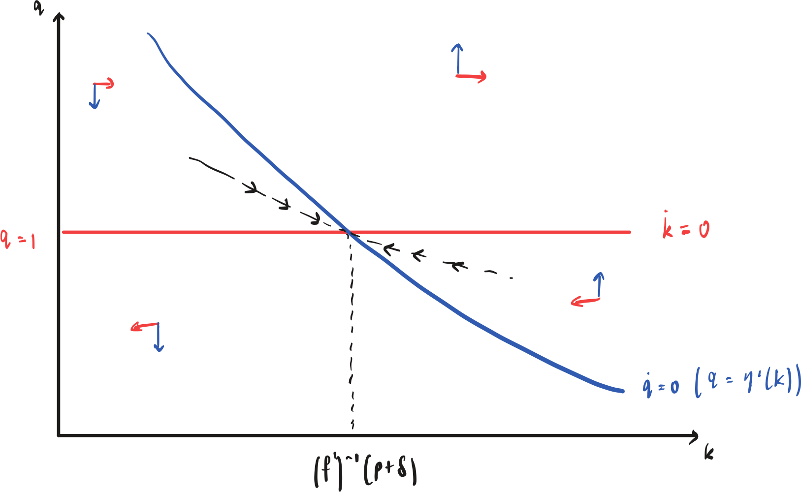
where f is strictly increasing, strictly concave, and satisfies the Inada conditions. The constraint 0≤i≤f(k) is the (linear) adjustment cost: investment can be neither negative nor larger than output. The Hamiltonian is
H(k,i,q)=f(k)−i+q(i−δk)
Since H is linear in the control with slope Hi=q−1, maximizing over i∈[0,f(k)] yields a bang-bang policy with three cases,
iii=0∈[0,f(k)]=f(k)if q<1if q=1if q>1
The remaining first order conditions are
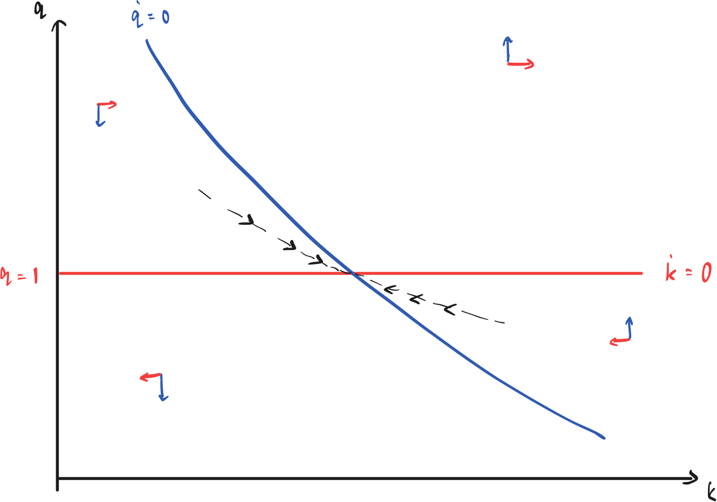
q˙k˙=ρq−Hk=(ρ+δ)q−f′(k)=i−δk
The k˙=0 locus is the horizontal line q=1 (where interior i=δk is admissible), and the q˙=0 locus is q=f′(k)/(ρ+δ), which is downward sloping by concavity of f. The phase diagram is below.
where k∗ solves f′(k∗)=ρ+δ. Along the saddle path of the phase diagram, q and k move together so that
k=k∗k<k∗k>k∗⟺q=1⟺Hi=0⟺q>1⟺Hi>0⟺q<1⟺Hi<0
which is exactly the sign pattern that makes u optimal: Hi<0 calls for i=0, Hi>0 for i=f(k), and Hi=0 leaves i interior. The system can therefore be solved recursively. First solve the autonomous law of motion
k˙=u(k)−δk
forward from k(0).[1] Given the path k(t), the costate solves the linear equation q˙−(ρ+δ)q=−f′(k). Multiplying by the integrating factor e−(ρ+δ)t,
with no restriction on i. The quantity iϕ(i/k) is the total adjustment cost incurred over and above the purchase price i of the investment good. We assume
The bracketed term f′(k)−x(1+ϕ(x)) is the marginal benefit of investing: the marginal product of capital net of the per-unit-of-capital cost of investment (purchase plus adjustment). This linear equation in q solves forward to
which one verifies by differentiating in t. Thus q(t) is the present value of the marginal benefits of capital, discounted at the effective rate ρ+δ−x. The adjustment to the discount rate appears because k˙/k=x−δ is the proportional growth rate of capital.
around (q,k)=(1,k∗), using γ(1)=δ and γ′(1)=1/θ′(δ)=1/(2ϕ′(δ)+δϕ′′(δ)). For the costate, the q-derivative of γ(q)2ϕ′(γ(q)) evaluated at q=1 is, exactly as in the η′ computation,
Let ζ=2ϕ′(δ)+δϕ′′(δ) measure the curvature of the adjustment technology. Then ∣λ−∣ is increasing in ε and decreasing in ζ: convergence is faster when the production function is more concave (a larger loss from being away from the steady state) and slower when adjustment costs are steeper. Diagonalizing H=Φ−1ΘΦ and setting z=Φ[q^,k^]′ gives z˙=Θz, so the stable mode decays at rate ∣λ−∣ and convergence is faster the larger ∣λ−∣ is.
If −f′′ increases (i.e. ε↑), then s′↓: the saddle path steepens and, as we saw, capital converges faster. As f′′→0 (ε→0), s′→0 and convergence becomes extremely slow: a change in the capital stock brings no change in productivity, so q stays near 1 and there is almost no force pulling capital toward k∗.
The dependence on ζ takes more care. To organize the algebra, write
R≡(ρ2+ζ4(ρ+δ)ε)1/2,s′=2k∗ζ(ρ−R)
so that R2−ρ2=4(ρ+δ)ε/ζ and dR/dζ=2R1⋅(−4(ρ+δ)ε/ζ2)=−2(ρ+δ)ε/(ζ2R). By the product rule,
since s′<0 and R>ρ>0. The saddle path steepens as ζ rises.
The two limits are instructive. Writing ρ−R=(ρ2−R2)/(ρ+R)=−4(ρ+δ)ε/(ζ(ρ+R)),
s′=2k∗ζ(ρ−R)=−k∗(ρ+R)2(ρ+δ)ε
As ζ→0, R→∞ and s′→0: with negligible adjustment costs capital jumps essentially instantaneously to k∗ while q stays at 1, so the saddle path is horizontal. As ζ→∞, R→ρ, and using (ρ+δ)ε=−k∗f′′(k∗),
s′→−k∗⋅2ρ2(ρ+δ)ε=−k∗ρ(ρ+δ)ε=ρf′′(k∗)=η′(k∗)
the saddle path approaches the q˙=0 locus: when adjustment is prohibitively costly the economy crawls along the η locus, and convergence (governed by ∣λ−∣→0) is very slow even though the path itself is steep.
Since q(k)=V′(k) and q>0, the value function is increasing. Along the saddle path q(k)=s(k) with s′<0, so V′′(k)=q′(k)=s′(k)<0 and V is concave. The ratio V(k)/k is the market (book) value of capital per unit installed — the firm’s stock price — i.e. the average value of capital, while q(k)=V′(k) is the marginal value of an additional unit. Thus V(k)/k is average q and q(k) is marginal q.
Finally suppose f(k)=πk. This arises from an underlying neoclassical production function F(k,l) that is homogeneous of degree one, strictly quasi-concave, and satisfies the Inada conditions. Given the capital stock, the firm chooses labor to maximize sales net of the wage bill,
lmaxF(k,l)−wl
with first order condition Fl(k,l)=w. Because F is homogeneous of degree one, its partials are homogeneous of degree zero, so Fl(k,l)=Fl(1,l/k), and the optimal labor-capital ratio l/k=λ(w) solves w=Fl(1,λ(w)). Euler’s theorem gives F(k,l)=Fk(k,l)k+Fl(k,l)l, and applying degree-zero homogeneity to each partial,
If k is restricted to a suitable region so that γ stays below ρ+δ, this condition holds; in particular it holds in a neighborhood of the steady state, where γ=δ<ρ+δ. Globally the map need not be single-valued: as k→0 the Inada condition forces f′(k)→∞, hence q→∞ and x=γ(q)→∞, so x crosses ρ+δ at a finite k~<k∗ where the locus folds and η′ blows up.